Thermochemical comparison of fuels

This notebook compares the thermal behavior of three fuels of interest in energy systems, using pyglenn:

Species	Fuel
CH4	Methane (natural gas / biogas)
C2H5OH	Ethanol (biofuel)
C3H8	Propane (LPG)

We will visualize \(C_p(T)\), \(S^\circ(T)\) and the sensible enthalpy change \(\Delta H(298.15\,\mathrm{K} \to T)\) over a temperature range relevant to combustion.

Requires matplotlib — install with pip install -e ".[examples]".

import matplotlib.pyplot as plt

from pyglenn import ThermochemicalCalculator

FUELS = {
    'CH4': 'Methane (natural gas)',
    'C2H5OH': 'Ethanol',
    'C3H8': 'Propane (LPG)',
}

Resolving the identifiers

get_available_species matches by substring, so we filter by exact name and gas phase to get the correct id for each species.

def resolve_id(calc, name, phase='gas'):
    """Return the id of the species with the exact name and phase."""
    for s in calc.get_available_species(name):
        if s['name'] == name and s['phase'] == phase:
            return s['id']
    raise ValueError(f'Species {name!r} ({phase}) not found')


with ThermochemicalCalculator() as calc:
    ids = {name: resolve_id(calc, name) for name in FUELS}

for name, sid in ids.items():
    print(f'{name:8} -> id {sid}')

CH4      -> id 296
C2H5OH   -> id 370
C3H8     -> id 393

Collecting properties over 300–2000 K

We use get_properties_range to evaluate all temperatures at once. The 300–2000 K range spans from ambient conditions up to typical flames.

temperatures = list(range(300, 2001, 50))

data = {}
with ThermochemicalCalculator() as calc:
    for name, sid in ids.items():
        span = calc.get_properties_range(sid, temperatures)
        Ts = sorted(span)
        data[name] = {
            'T': Ts,
            'cp': [span[T]['cp'] for T in Ts],
            's': [span[T]['s'] for T in Ts],
        }
        # Sensible ΔH relative to 298.15 K
        data[name]['dh'] = [
            calc.calculate_enthalpy_change(sid, 298.15, T) / 1000.0 for T in Ts
        ]  # kJ/mol

print('Properties collected for:', ', '.join(data))

Properties collected for: CH4, C2H5OH, C3H8

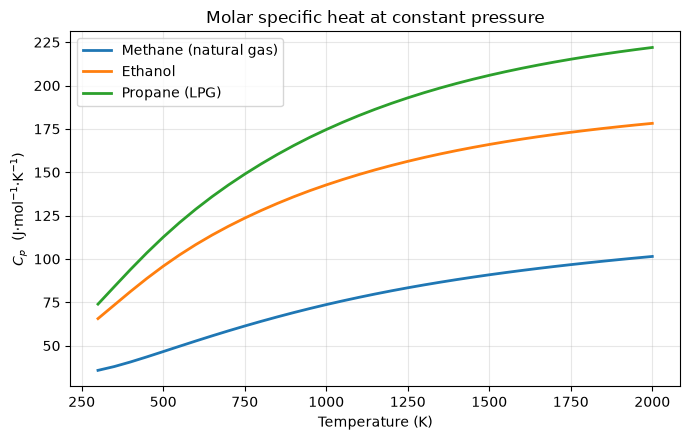
Specific heat \(C_p(T)\)

\(C_p\) rises with temperature as more vibrational modes become active. Larger molecules (ethanol, propane) have higher \(C_p\) because they have more degrees of freedom.

fig, ax = plt.subplots(figsize=(7, 4.5))
for name, d in data.items():
    ax.plot(d['T'], d['cp'], label=FUELS[name], linewidth=2)
ax.set_xlabel('Temperature (K)')
ax.set_ylabel(r'$C_p$  (J·mol$^{-1}$·K$^{-1}$)')
ax.set_title('Molar specific heat at constant pressure')
ax.legend()
ax.grid(True, alpha=0.3)
fig.tight_layout()
plt.show()

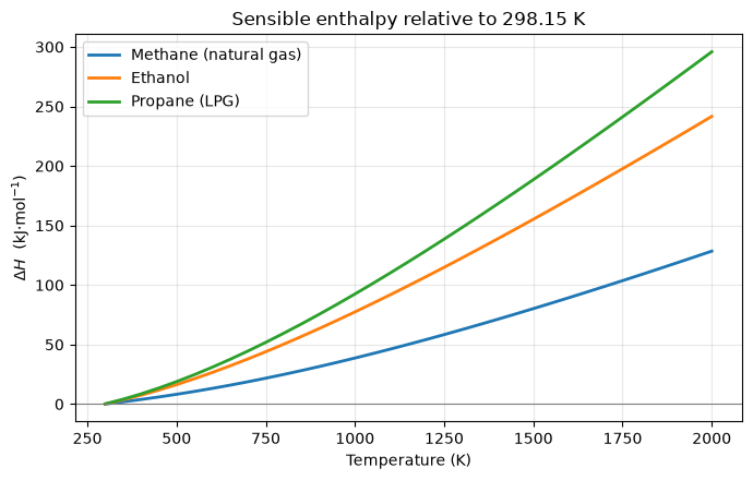
Sensible enthalpy \(\Delta H(298.15\,\mathrm{K} \to T)\)

This is the heat required to warm 1 mol of fuel from 298.15 K up to \(T\) — a central quantity in energy balances for preheating and heat recovery (HRSG).

fig, ax = plt.subplots(figsize=(7, 4.5))
for name, d in data.items():
    ax.plot(d['T'], d['dh'], label=FUELS[name], linewidth=2)
ax.axhline(0, color='gray', linewidth=0.8)
ax.set_xlabel('Temperature (K)')
ax.set_ylabel(r'$\Delta H$  (kJ·mol$^{-1}$)')
ax.set_title('Sensible enthalpy relative to 298.15 K')
ax.legend()
ax.grid(True, alpha=0.3)
fig.tight_layout()
plt.show()

Numerical summary at reference points

Direct comparison of \(C_p\) and \(S^\circ\) at three temperatures of interest.

targets = [300, 1000, 2000]

print(f"{'Fuel':<22} {'T (K)':>6} {'Cp':>10} {'S°':>10}")
print('-' * 50)
for name, d in data.items():
    for T in targets:
        i = d['T'].index(T)
        print(f'{FUELS[name]:<22} {T:>6} {d["cp"][i]:>10.3f} {d["s"][i]:>10.3f}')
    print()

Fuel                    T (K)         Cp         S°
--------------------------------------------------
Methane (natural gas)     300     35.760    186.591
Methane (natural gas)    1000     73.676    248.330
Methane (natural gas)    2000    101.442    309.447

Ethanol                   300     65.593    280.996
Ethanol                  1000    142.689    404.550
Ethanol                  2000    178.201    516.949

Propane (LPG)             300     73.955    270.770
Propane (LPG)            1000    174.613    417.339
Propane (LPG)            2000    221.955    556.442

Reading the results

• Ethanol and propane, being larger molecules, show higher \(C_p\) and \(S^\circ\) than methane across the whole range.

• The sensible enthalpy grows almost linearly at high temperatures, reflecting the plateau of \(C_p\).

• These data feed energy balances in combustion chambers, gasifiers and power cycles — see the applications in the project README.