02 - NASA Polynomials Under the Hood
Notebook 01 treated calculate_properties as a black box. Here we open it up and reproduce every number from the raw polynomial coefficients stored in the database.
pyglenn uses the NASA Glenn 9-coefficient functional form. Over each temperature interval the three standard-state properties are
The seven \(a_i\) fix the shape of \(C_p(T)\); the two integration constants \(b_1\) and \(b_2\) set the enthalpy and entropy references, respectively. We will see that \(b_1\) is what makes \(H^\circ(T)\) carry the enthalpy of formation.
[1]:
from pyglenn import ThermochemicalCalculator, R

print("Universal gas constant R =", R, "J/(mol.K)")
Universal gas constant R = 8.314462618 J/(mol.K)
[2]:
%matplotlib inline
import numpy as np
import matplotlib.pyplot as plt
import pandas as pd

plt.rcParams["figure.figsize"] = (8, 4.5)
plt.rcParams["axes.grid"] = True
pd.set_option("display.float_format", lambda v: f"{v:,.3f}")

import math
from pyglenn import ThermoDBQuery
1. The raw data for a species
calc.db.get_species_data(id) returns the full record for a species, including one entry per temperature interval with its coefficient set. Let’s look at molecular oxygen.
[3]:
with ThermochemicalCalculator() as calc:
    o2 = calc.get_available_species("O2", exact_match=True)[0]["id"]
    data = calc.db.get_species_data(o2)

print("Species  :", data["name"])
print("Phase    :", data["phase"])
print("M        :", data["molecular_weight"], "g/mol")
print("Intervals:", len(data["intervals"]))
for iv in data["intervals"]:
    print(f"   #{iv['interval_number']}: {iv['temp_min']:6.0f} - {iv['temp_max']:6.0f} K")
Species  : O2
Phase    : gas
M        : 31.9988 g/mol
Intervals: 3
   #1:    200 -   1000 K
   #2:   1000 -   6000 K
   #3:   6000 -  20000 K
Each interval carries its own nine coefficients. Displaying them side by side shows how the fit is split across the temperature range.
[4]:
rows = []
for iv in data["intervals"]:
    row = {"T_min": iv["temp_min"], "T_max": iv["temp_max"]}
    row.update(iv["coefficients"])
    rows.append(row)

coef_df = pd.DataFrame(rows).set_index(["T_min", "T_max"])
with pd.option_context("display.float_format", lambda v: f"{v: .6e}"):
    print(coef_df.to_string())
                                     a1            a2            a3            a4            a5            a6            a7            b1            b2
T_min        T_max
2.000000e+02 1.000000e+03 -3.425563e+04  4.847001e+02  1.119011e+00  4.293889e-03 -6.836301e-07 -2.023373e-09  1.039040e-12 -3.391455e+03  1.849699e+01
1.000000e+03 6.000000e+03 -1.037939e+06  2.344830e+03  1.819732e+00  1.267848e-03 -2.188068e-07  2.053720e-11 -8.193467e-16 -1.689011e+04  1.738717e+01
6.000000e+03 2.000000e+04  4.975294e+08 -2.866107e+05  6.690352e+01 -6.169959e-03  3.016396e-07 -7.421417e-12  7.278176e-17  2.293554e+06 -5.530622e+02
2. Reconstructing the properties by hand
We now implement the three formulas literally and compare against the library. pyglenn also exposes them as static methods on ThermoDBQuery (calculate_cp, calculate_h, calculate_s), which return the dimensionless groups \(C_p/R\), \(H/RT\) and \(S/R\).
[5]:
def cp_over_R(c, T):
    return (c["a1"]/T**2 + c["a2"]/T + c["a3"] + c["a4"]*T
            + c["a5"]*T**2 + c["a6"]*T**3 + c["a7"]*T**4)

def h_over_RT(c, T):
    return (-c["a1"]/T**2 + c["a2"]*math.log(T)/T + c["a3"] + c["a4"]*T/2
            + c["a5"]*T**2/3 + c["a6"]*T**3/4 + c["a7"]*T**4/5 + c["b1"]/T)

def s_over_R(c, T):
    return (-c["a1"]/(2*T**2) - c["a2"]/T + c["a3"]*math.log(T) + c["a4"]*T
            + c["a5"]*T**2/2 + c["a6"]*T**3/3 + c["a7"]*T**4/4 + c["b2"])
[6]:
T = 1000.0
with ThermochemicalCalculator() as calc:
    o2 = calc.get_available_species("O2", exact_match=True)[0]["id"]
    interval = calc.db.get_species_for_temperature(o2, T)   # picks the right piece
    c = interval["coefficients"]
    api = calc.calculate_properties(o2, T)

cp_manual = cp_over_R(c, T) * R           # J/(mol.K)
h_manual  = h_over_RT(c, T) * R * T       # J/mol
s_manual  = s_over_R(c, T) * R            # J/(mol.K)

print(f"{'':10s}{'manual':>16s}{'pyglenn API':>16s}")
print(f"{'Cp':10s}{cp_manual:16.6f}{api['cp']:16.6f}")
print(f"{'H':10s}{h_manual:16.4f}{api['h_relative']:16.4f}")
print(f"{'S':10s}{s_manual:16.6f}{api['s']:16.6f}")

assert np.isclose(cp_manual, api["cp"])
assert np.isclose(h_manual, api["h_relative"])
assert np.isclose(s_manual, api["s"])
print("\nManual reconstruction matches the API to floating-point precision.")
                    manual     pyglenn API
Cp               34.882346       34.882346
H               22707.0813      22707.0813
S               243.585926      243.585926

Manual reconstruction matches the API to floating-point precision.
And the static helpers return exactly the dimensionless groups our functions compute:
[7]:
print("Cp/R :", ThermoDBQuery.calculate_cp(c, T), "==", cp_over_R(c, T))
print("H/RT :", ThermoDBQuery.calculate_h(c, T),  "==", h_over_RT(c, T))
print("S/R  :", ThermoDBQuery.calculate_s(c, T),  "==", s_over_R(c, T))
Cp/R : 4.195381929800001 == 4.195381929800001
H/RT : 2.7310341435749046 == 2.7310341435749046
S/R  : 29.296652945019957 == 29.296652945019957
Dimensionless vs. absolute
The dimensionless groups are what the polynomial produces; multiplying by \(R\) (and by \(T\) for enthalpy) gives SI units.
[8]:
summary = pd.DataFrame({
    "dimensionless": [cp_over_R(c, T), h_over_RT(c, T), s_over_R(c, T)],
    "multiplier":    ["x R", "x R T", "x R"],
    "absolute":      [api["cp"], api["h_relative"], api["s"]],
    "units":         ["J/(mol.K)", "J/mol", "J/(mol.K)"],
}, index=["Cp", "H", "S"])
print(summary.to_string())
    dimensionless multiplier   absolute      units
Cp          4.195        x R     34.882  J/(mol.K)
H           2.731      x R T 22,707.081      J/mol
S          29.297        x R    243.586  J/(mol.K)
3. The piecewise structure
pyglenn selects the piece that contains the requested temperature. Around the 1000 K boundary of O₂ the temp_interval field switches, yet \(C_p\) stays continuous — the NASA fits are constrained to match at the seams.
[9]:
with ThermochemicalCalculator() as calc:
    o2 = calc.get_available_species("O2", exact_match=True)[0]["id"]
    for T in [999.0, 1000.0, 1001.0]:
        p = calc.calculate_properties(o2, T)
        print(f"T = {T:7.1f} K  ->  Cp = {p['cp']:.5f} J/(mol.K)  "
              f"(interval {p['temp_interval']})")
T =   999.0 K  ->  Cp = 34.87739 J/(mol.K)  (interval [200.0, 1000.0])
T =  1000.0 K  ->  Cp = 34.88235 J/(mol.K)  (interval [200.0, 1000.0])
T =  1001.0 K  ->  Cp = 34.88749 J/(mol.K)  (interval [1000.0, 6000.0])
4. What \(b_1\) and \(b_2\) encode
The heat-capacity coefficients \(a_1\ldots a_7\) are obtained first by fitting \(C_p(T)\). Integrating \(C_p\) leaves one constant for enthalpy and one for entropy — these are \(b_1\) and \(b_2\). NASA chooses them so that \(H^\circ(T)\) is on the standardized scale (it already includes the enthalpy of formation) and \(S^\circ(T)\) is the absolute (Third-Law) entropy. We can see \(b_1\)’s effect directly: elements sit at ≈ 0, compounds carry \(\Delta_f H^\circ\).
[10]:
with ThermochemicalCalculator() as calc:
    for name in ["O2", "N2", "H2", "H2O", "CO2"]:
        sid = calc.get_available_species(name, exact_match=True)[0]["id"]
        h298 = calc.calculate_properties(sid, 298.15)["h_relative"]
        print(f"{name:5s}  H(298.15 K) = {h298/1000:9.3f} kJ/mol")
O2     H(298.15 K) =    -0.000 kJ/mol
N2     H(298.15 K) =     0.000 kJ/mol
H2     H(298.15 K) =    -0.000 kJ/mol
H2O    H(298.15 K) =  -241.825 kJ/mol
CO2    H(298.15 K) =  -393.508 kJ/mol
5. Visualising the fit
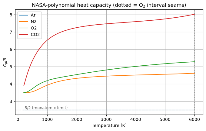
We plot the dimensionless heat capacity \(C_p/R\) for a monatomic gas (Ar), two diatomics (O₂, N₂) and a triatomic (CO₂), marking O₂’s interval boundaries. The monatomic gas is flat at \(5/2\); the polyatomics climb as vibrational modes activate — physics we revisit in notebook 03.
[11]:
Tgrid = np.linspace(200, 6000, 400)
fig, ax = plt.subplots()
with ThermochemicalCalculator() as calc:
    for name in ["Ar", "N2", "O2", "CO2"]:
        sid = calc.get_available_species(name, exact_match=True)[0]["id"]
        cp_r = [calc.calculate_properties(sid, T)["cp"] / R for T in Tgrid]
        ax.plot(Tgrid, cp_r, label=name)
for boundary in (1000.0, 6000.0):
    ax.axvline(boundary, ls=":", color="0.6")
ax.axhline(2.5, ls="--", color="0.7")
ax.text(230, 2.55, "5/2 (monatomic limit)", fontsize=9, color="0.4")
ax.set_xlabel("Temperature [K]")
ax.set_ylabel(r"$C_p / R$")
ax.set_title("NASA-polynomial heat capacity (dotted = O$_2$ interval seams)")
ax.legend()
plt.show()
6. Validation against known values
A final sanity check against textbook standard-state values for O₂ at 298.15 K (\(C_p^\circ = 29.378\) J/mol/K, \(S^\circ = 205.15\) J/mol/K).
[12]:
with ThermochemicalCalculator() as calc:
    p = calc.calculate_properties(calc.get_available_species("O2", exact_match=True)[0]["id"], 298.15)
for label, got, ref in [("Cp", p["cp"], 29.378), ("S", p["s"], 205.15)]:
    print(f"{label}: pyglenn = {got:8.3f}   reference = {ref:8.3f}   "
          f"rel.err = {abs(got-ref)/ref*100:.3f}%")
Cp: pyglenn =   29.378   reference =   29.378   rel.err = 0.001%
S: pyglenn =  205.148   reference =  205.150   rel.err = 0.001%
Summary
pyglennstores NASA Glenn 9-term coefficients, piecewise in temperature.calculate_propertiesselects the right interval and evaluates the three closed-form expressions — which we reproduced by hand exactly.\(b_1\) puts \(H^\circ\) on the standardized scale (carrying \(\Delta_f H^\circ\)); \(b_2\) sets the absolute-entropy reference.
Next: notebook 03 turns these formulas into property curves and connects their shape to molecular structure.