03 - Temperature-Dependent Properties & Plotting
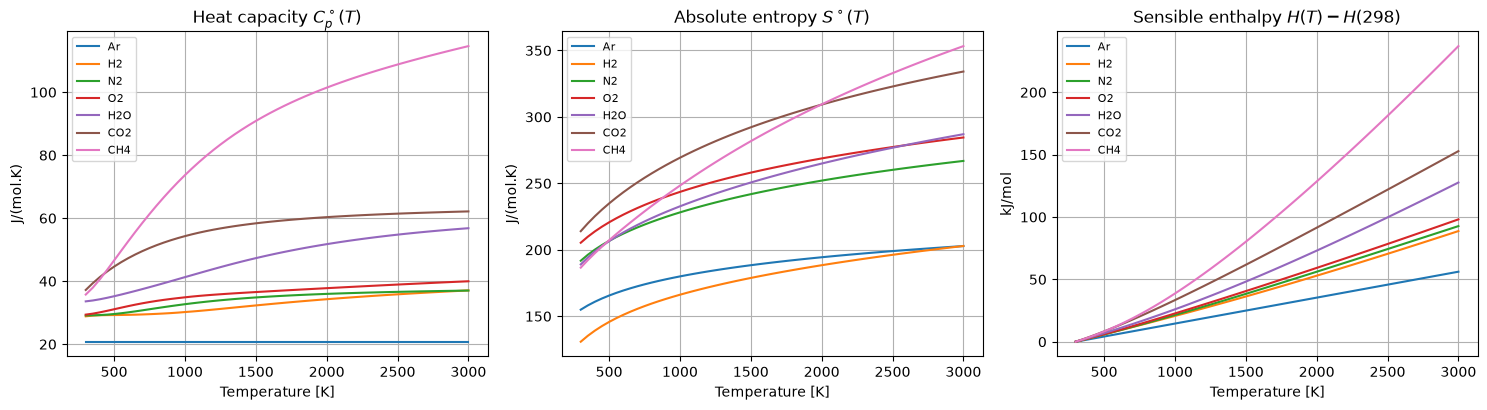
A constant heat capacity is a fine approximation over a narrow temperature window, but combustion, gas turbines and reacting flows span hundreds — even thousands — of kelvin. There \(C_p\), \(S^\circ\) and \(H^\circ\) vary strongly, and pyglenn gives you their true temperature dependence directly from the NASA polynomials.
In this notebook we
sweep temperature and build property curves for several gases;
read the physics off the \(C_p(T)\) curves (equipartition and vibrations);
tabulate the results with
pandas;contrast the instantaneous and mean heat capacities; and
see how condensed phases have narrower validity ranges.
[1]:
from pyglenn import ThermochemicalCalculator, R

print("Universal gas constant R =", R, "J/(mol.K)")
Universal gas constant R = 8.314462618 J/(mol.K)
[2]:
%matplotlib inline
import numpy as np
import matplotlib.pyplot as plt
import pandas as pd

plt.rcParams["figure.figsize"] = (8, 4.5)
plt.rcParams["axes.grid"] = True
pd.set_option("display.float_format", lambda v: f"{v:,.3f}")
1. Sweeping temperature
get_properties_range(id, temps) evaluates a whole list of temperatures at once and returns a dict keyed by temperature. We wrap it in a small helper that returns arrays ready for plotting, skipping any temperature that falls outside the species’ validity range (those come back missing).
[3]:
SPECIES = ["Ar", "H2", "N2", "O2", "H2O", "CO2", "CH4"]

def curve(calc, name, temps):
    """Return (T, cp, s, h) arrays for the temperatures that are in range."""
    sid = calc.get_available_species(name, exact_match=True)[0]["id"]
    table = calc.get_properties_range(sid, list(temps)) or {}
    T = np.array(sorted(table))
    cp = np.array([table[t]["cp"] for t in T])
    s = np.array([table[t]["s"] for t in T])
    h = np.array([table[t]["h_relative"] for t in T])
    return T, cp, s, h

temps = np.linspace(300, 3000, 55)
data = {}
with ThermochemicalCalculator() as calc:
    for name in SPECIES:
        data[name] = curve(calc, name, temps)
print("Computed curves for:", ", ".join(data))
Computed curves for: Ar, H2, N2, O2, H2O, CO2, CH4
2. Three property curves
\(C_p^\circ(T)\), \(S^\circ(T)\) and the sensible enthalpy \(H^\circ(T)-H^\circ(298.15\,\mathrm{K})\) (the enthalpy needed to heat the species from room temperature). We subtract the 298.15 K value so every curve starts near zero and the shapes are comparable regardless of formation enthalpy.
[4]:
fig, axes = plt.subplots(1, 3, figsize=(15, 4.2))
with ThermochemicalCalculator() as calc:
    h_ref = {n: calc.calculate_properties(calc.get_available_species(n, exact_match=True)[0]["id"], 298.15)["h_relative"]
             for n in SPECIES}

for name in SPECIES:
    T, cp, s, h = data[name]
    axes[0].plot(T, cp, label=name)
    axes[1].plot(T, s, label=name)
    axes[2].plot(T, (h - h_ref[name]) / 1000.0, label=name)

axes[0].set_title(r"Heat capacity $C_p^\circ(T)$"); axes[0].set_ylabel("J/(mol.K)")
axes[1].set_title(r"Absolute entropy $S^\circ(T)$"); axes[1].set_ylabel("J/(mol.K)")
axes[2].set_title("Sensible enthalpy $H(T)-H(298)$"); axes[2].set_ylabel("kJ/mol")
for ax in axes:
    ax.set_xlabel("Temperature [K]"); ax.legend(fontsize=8)
fig.tight_layout()
plt.show()
3. Reading the physics: equipartition
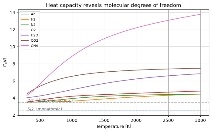
The dimensionless heat capacity \(C_p/R\) exposes molecular structure. By equipartition, each fully active quadratic degree of freedom contributes \(\tfrac12 R\) to \(C_v\), and for an ideal gas \(C_p = C_v + R\):
Monatomic (Ar): only 3 translational modes \(\Rightarrow C_v=\tfrac32 R\), so \(C_p=\tfrac52 R\) — flat at all temperatures.
Diatomic (N₂, O₂, H₂): + 2 rotational modes \(\Rightarrow C_p=\tfrac72 R\) at moderate \(T\), rising further as the vibrational mode switches on.
Polyatomic (CO₂, H₂O, CH₄): more rotational and many vibrational modes, so \(C_p/R\) is larger and climbs steeply.
The dashed lines mark the \(\tfrac52\) and \(\tfrac72\) plateaus.
[5]:
fig, ax = plt.subplots()
for name in SPECIES:
    T, cp, s, h = data[name]
    ax.plot(T, cp / R, label=name)
for level, txt in [(2.5, "5/2  (monatomic)"), (3.5, "7/2  (diatomic, no vib.)")]:
    ax.axhline(level, ls="--", color="0.7")
    ax.text(310, level + 0.05, txt, fontsize=9, color="0.4")
ax.set_xlabel("Temperature [K]")
ax.set_ylabel(r"$C_p / R$")
ax.set_title("Heat capacity reveals molecular degrees of freedom")
ax.legend(fontsize=8)
plt.show()
4. A property table with pandas
Discrete tables are still handy for reports. Here is \(C_p\) at a set of temperatures for every species, sorted by the value at 2000 K to rank them by how much energy they soak up when hot.
[6]:
table_temps = [300, 600, 1000, 1500, 2000, 2500]
records = {}
with ThermochemicalCalculator() as calc:
    for name in SPECIES:
        sid = calc.get_available_species(name, exact_match=True)[0]["id"]
        records[name] = {f"{t} K": calc.calculate_properties(sid, t)["cp"]
                         for t in table_temps}

cp_df = pd.DataFrame(records).T.sort_values("2000 K", ascending=False)
cp_df.index.name = "species"
print("Cp [J/(mol.K)]")
print(cp_df.to_string())
Cp [J/(mol.K)]
         300 K  600 K  1000 K  1500 K  2000 K  2500 K
species
CH4     35.760 52.690  73.676  90.865 101.442 108.789
CO2     37.220 47.322  54.308  58.374  60.334  61.443
H2O     33.596 36.324  41.291  47.318  51.755  54.777
O2      29.387 32.090  34.882  36.553  37.784  38.933
N2      29.125 30.109  32.696  34.842  35.970  36.615
H2      28.849 29.318  30.206  32.304  34.276  35.832
Ar      20.786 20.786  20.786  20.786  20.786  20.786
5. Instantaneous vs. mean heat capacity
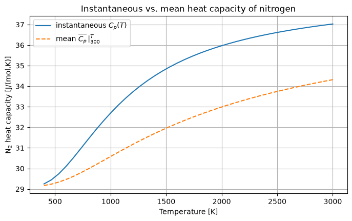
Two heat capacities appear in engineering calculations:
the instantaneous \(C_p(T) = \left(\partial H/\partial T\right)_p\);
the mean \(\overline{C_p}\big|_{T_1}^{T_2} = \dfrac{H(T_2)-H(T_1)}{T_2-T_1}\), which is what you actually multiply by \(\Delta T\) to get an enthalpy change.
Using calculate_enthalpy_change for the numerator, we compare the two for nitrogen. The mean (from 300 K) lags the instantaneous value because it averages in the cooler, lower-\(C_p\) region.
[7]:
T2 = np.linspace(400, 3000, 40)
with ThermochemicalCalculator() as calc:
    n2 = calc.get_available_species("N2", exact_match=True)[0]["id"]
    cp_inst = np.array([calc.calculate_properties(n2, t)["cp"] for t in T2])
    cp_mean = np.array([calc.calculate_enthalpy_change(n2, 300.0, t) / (t - 300.0)
                        for t in T2])

fig, ax = plt.subplots()
ax.plot(T2, cp_inst, label=r"instantaneous $C_p(T)$")
ax.plot(T2, cp_mean, "--", label=r"mean $\overline{C_p}\,|_{300}^{T}$")
ax.set_xlabel("Temperature [K]")
ax.set_ylabel("N$_2$ heat capacity [J/(mol.K)]")
ax.set_title("Instantaneous vs. mean heat capacity of nitrogen")
ax.legend()
plt.show()
6. Condensed phases have narrower ranges
Gas-phase fits typically cover 200–6000 K, but liquids and solids are only valid over a small window. Requesting a temperature outside that window raises a TemperatureOutOfRangeError — catch it with try/except. Liquid water is a good example.
[ ]:
from pyglenn import TemperatureOutOfRangeError

with ThermochemicalCalculator() as calc:
    liq = calc.get_available_species("H2O(L)", exact_match=True)[0]["id"]
    data_liq = calc.db.get_species_data(liq)
    ranges = [(iv["temp_min"], iv["temp_max"]) for iv in data_liq["intervals"]]
    print("H2O(L) valid interval(s):", ranges)
    for T in [350.0, 2000.0]:
        try:
            p = calc.calculate_properties(liq, T)
            print(f"  T = {T:7.1f} K  ->  Cp = {p['cp']:.2f} J/(mol.K)")
        except TemperatureOutOfRangeError:
            print(f"  T = {T:7.1f} K  ->  out of range")
H2O(L) valid interval(s): [(273.15, 373.15), (373.15, 600.0)]
  T =   350.0 K  ->  Cp = 75.53 J/(mol.K)
---------------------------------------------------------------------------
TemperatureOutOfRangeError                Traceback (most recent call last)
Cell In[8], line 7
      3     data_liq = calc.db.get_species_data(liq)
      4     ranges = [(iv["temp_min"], iv["temp_max"]) for iv in data_liq["intervals"]]
      5     print("H2O(L) valid interval(s):", ranges)
      6     for T in [350.0, 2000.0]:
----> 7         p = calc.calculate_properties(liq, T)
      8         status = "None (out of range)" if p is None else f"Cp = {p['cp']:.2f} J/(mol.K)"
      9         print(f"  T = {T:7.1f} K  ->  {status}")

File ~\miniconda3\envs\ct-env\Lib\site-packages\pyglenn\calculator.py:192, in ThermochemicalCalculator.calculate_properties(self, species_id, temperature)
    188 if not interval_data:
    189     intervals = [
    190         (i['temp_min'], i['temp_max']) for i in species_data['intervals']
    191     ]
--> 192     raise TemperatureOutOfRangeError(
    193         f'Temperature {temperature:.1f} K out of valid range '
    194         f"for species '{species_data['name']}'. "
    195         f'Available intervals: {intervals}'
    196     )
    198 coeffs: dict[str, float] = interval_data['coefficients']
    200 # Dimensionless properties (÷ R)

TemperatureOutOfRangeError: Temperature 2000.0 K out of valid range for species 'H2O(L)'. Available intervals: [(273.15, 373.15), (373.15, 600.0)]
Summary
get_properties_rangesweeps many temperatures in one call.The shape of \(C_p/R\) directly reflects translational, rotational and vibrational degrees of freedom.
Mean and instantaneous \(C_p\) differ — use the mean (via
calculate_enthalpy_change) for finite \(\Delta T\).Always handle
Nonefor out-of-range temperatures, especially for condensed phases.
Next: notebook 04 extracts enthalpies of formation from these same polynomials.