09 - Brayton Gas-Turbine Cycle
The Brayton cycle is the thermodynamic backbone of gas-turbine engines for power generation and jet propulsion. The air-standard idealisation comprises four processes:
Isentropic compression (compressor): \(P_1 \to P_2 = r_p P_1\)
Isobaric heat addition (combustor): \(T_2 \to T_3\)
Isentropic expansion (turbine): \(P_3 \to P_4 = P_3 / r_p\)
Isobaric heat rejection (exhaust)
Textbook analysis assumes constant \(C_p\) and \(\gamma = C_p/C_v\), giving the familiar efficiency \(\eta = 1 - r_p^{(1-\gamma)/\gamma}\). Here we use pyglenn’s real \(C_p(T)\) and \(S^\circ(T)\) — the working fluid is a real-gas mixture of O₂ and N₂ (air) — and solve the isentropic \(S(T_2) = S(T_1)\) condition numerically.
The thermal efficiency follows directly from the enthalpy values at each state:
[1]:
from pyglenn import ThermochemicalCalculator, R

print("Universal gas constant R =", R, "J/(mol.K)")
Universal gas constant R = 8.314462618 J/(mol.K)
[2]:
%matplotlib inline
import numpy as np
import matplotlib.pyplot as plt
import pandas as pd

plt.rcParams["figure.figsize"] = (8, 4.5)
plt.rcParams["axes.grid"] = True
pd.set_option("display.float_format", lambda v: f"{v:,.3f}")

from scipy.optimize import brentq
1. Air as the working fluid
We model dry air as the mixture \(1\ \mathrm{O_2} + 3.76\ \mathrm{N_2}\). Single-species functions for enthalpy and entropy of the mixture follow.
[3]:
AIR = {"O2": 1.0, "N2": 3.76}
R_UNIV = R  # J/(mol·K) — universal gas constant

def air_enthalpy(calc, T):
    """Total standardized enthalpy of 1 mol air at T, in J."""
    return sum(n * calc.calculate_properties(calc.get_available_species(name, exact_match=True)[0]["id"], T)["h_relative"]
               for name, n in AIR.items())

def air_entropy_std(calc, T):
    """Standard-state (P=1 bar) entropy of 1 mol air at T, in J/K."""
    return sum(n * calc.calculate_properties(calc.get_available_species(name, exact_match=True)[0]["id"], T)["s"]
               for name, n in AIR.items())

# Total moles in the mixture per mol of "air"
AIR_MOLES = sum(AIR.values())  # = 4.76
2. Isentropic relation with real \(C_p(T)\)
For an ideal gas the molar entropy at \((T,P)\) is
For an isentropic process (\(s_2 = s_1\)) between pressures \(P_1\) and \(P_2\), the pressure terms give \(s^\circ(T_2) - s^\circ(T_1) = R\ln(P_2/P_1)\). We solve
for \(T_2\) with a robust bracketed root-finder, accounting for the total moles in the air mixture.
[4]:
def isentropic_T(calc, T1, P_ratio):
    """Temperature after isentropic compression/expansion (P2/P1 = P_ratio).

    Returns T2 [K] such that s°(T2) - s°(T1) = R_air * ln(P2/P1),
    where R_air = R / M_air = R per mole of mixture times total moles.
    """
    s1 = air_entropy_std(calc, T1)
    R_air = R_UNIV * AIR_MOLES  # J/K per mol of air mixture
    target = s1 + R_air * np.log(P_ratio)

    def f(T):
        return air_entropy_std(calc, T) - target

    # Search bracket: entropy grows with T, so compression (P_ratio>1)
    # pushes T2 > T1; expansion (P_ratio<1) pushes T2 < T1.
    if P_ratio > 1:
        lo, hi = T1, T1 * (P_ratio ** 0.4 + 1)
    else:
        lo, hi = T1 * P_ratio ** 0.4, T1

    # Expand bracket if needed
    while f(lo) * f(hi) > 0:
        if P_ratio > 1:
            hi *= 1.3
        else:
            lo *= 0.7
        if hi > 6000 or lo < 50:
            raise RuntimeError(f"Could not bracket T2 for P_ratio={P_ratio}")

    return brentq(f, lo, hi)
3. Building the Brayton cycle
We set the cycle parameters:
Inlet: \(T_1 = 300\ \mathrm{K}\), \(P_1 = 1\ \mathrm{bar}\)
Pressure ratio: \(r_p = P_2/P_1 = 10\)
Turbine inlet temperature (TIT): \(T_3 = 1400\ \mathrm{K}\)
The four states are computed with real \(C_p(T)\) via the isentropic solver.
[5]:
def brayton_states(calc, T1, T3, rp):
    """Return dict of (T, h_per_kg_air) for the four Brayton states.

    h values are in kJ per kg of air (not per mole of mixture).
    """
    # Molecular weight of the air mixture (mole-weighted average)
    M_O2 = 31.9988   # g/mol
    M_N2 = 28.0134   # g/mol
    M_air = (AIR["O2"] * M_O2 + AIR["N2"] * M_N2) / AIR_MOLES  # g/mol

    T2 = isentropic_T(calc, T1, rp)          # compressor outlet
    T4 = isentropic_T(calc, T3, 1.0 / rp)    # turbine outlet

    def h_kJ_kg(T):
        return air_enthalpy(calc, T) / (M_air * 1e-3) / 1000  # kJ/kg

    return {
        "1 (compressor inlet)":  (T1, h_kJ_kg(T1)),
        "2 (compressor outlet)": (T2, h_kJ_kg(T2)),
        "3 (turbine inlet)":     (T3, h_kJ_kg(T3)),
        "4 (turbine outlet)":    (T4, h_kJ_kg(T4)),
    }

with ThermochemicalCalculator() as calc:
    states = brayton_states(calc, T1=300.0, T3=1400.0, rp=10)

print(f"{'State':<26s} {'T [K]':>8s} {'h [kJ/kg]':>12s}")
print("-" * 46)
for label, (T, h) in states.items():
    print(f"{label:<26s} {T:8.1f} {h:12.2f}")
State                         T [K]    h [kJ/kg]
----------------------------------------------
1 (compressor inlet)          300.0         8.91
2 (compressor outlet)         573.1      1344.35
3 (turbine inlet)            1400.0      5834.55
4 (turbine outlet)            789.3      2453.76
4. Thermal efficiency
We compare the real-gas result with the constant-\(\gamma\) textbook formula (\(\gamma \approx 1.4\) for diatomic air).
[6]:
T1, h1 = states["1 (compressor inlet)"]
T2, h2 = states["2 (compressor outlet)"]
T3, h3 = states["3 (turbine inlet)"]
T4, h4 = states["4 (turbine outlet)"]

w_comp = h2 - h1          # compressor work [kJ/kg]
w_turb = h3 - h4          # turbine work [kJ/kg]
q_in   = h3 - h2          # heat added [kJ/kg]
eta_real = (w_turb - w_comp) / q_in

# Cold air-standard (constant gamma = 1.4)
gamma = 1.4
rp = 10
eta_cold = 1 - rp ** ((1 - gamma) / gamma)

print(f"Real-gas Brayton efficiency  : {eta_real:.4f} ({eta_real*100:.1f}%)")
print(f"Cold air-standard (gamma=1.4): {eta_cold:.4f} ({eta_cold*100:.1f}%)")
print(f"Turbine work : {w_turb:.1f} kJ/kg")
print(f"Compressor work: {w_comp:.1f} kJ/kg")
print(f"Net work      : {w_turb - w_comp:.1f} kJ/kg")
Real-gas Brayton efficiency  : 0.4555 (45.6%)
Cold air-standard (gamma=1.4): 0.4821 (48.2%)
Turbine work : 3380.8 kJ/kg
Compressor work: 1335.4 kJ/kg
Net work      : 2045.3 kJ/kg
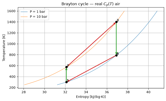
5. T–s diagram (qualitative)
We sketch the four states on temperature–entropy axes, using the standard entropy of the air mixture at each state pressure.
[7]:
def air_s_at_P(calc, T, P_bar):
    """Entropy of air mixture at (T, P), in kJ/(kg·K)."""
    s_std = air_entropy_std(calc, T)           # J/K per mol mixture
    R_air = R_UNIV * AIR_MOLES                  # J/K per mol mixture
    s_p = s_std - R_air * np.log(P_bar / 1.0)  # J/K per mol mixture
    M_air = (AIR["O2"] * 31.9988 + AIR["N2"] * 28.0134) / AIR_MOLES
    return s_p / (M_air * 1e-3) / 1000          # kJ/(kg·K)

rp = 10
T1_val, T3_val = 300.0, 1400.0

with ThermochemicalCalculator() as calc:
    T2_val = isentropic_T(calc, T1_val, rp)
    T4_val = isentropic_T(calc, T3_val, 1.0 / rp)

    # Isobars at P=1 bar and P=10 bar
    T_range = np.linspace(250, 1600, 100)
    s_low   = np.array([air_s_at_P(calc, T, 1)  for T in T_range])
    s_high  = np.array([air_s_at_P(calc, T, 10) for T in T_range])

    # The four states
    s1 = air_s_at_P(calc, T1_val, 1)
    s2 = air_s_at_P(calc, T2_val, 10)
    s3 = air_s_at_P(calc, T3_val, 10)
    s4 = air_s_at_P(calc, T4_val, 1)

fig, ax = plt.subplots()
ax.plot(s_low,  T_range, "C0", lw=0.8, label="P = 1 bar")
ax.plot(s_high, T_range, "C1", lw=0.8, label="P = 10 bar")
# Process arrows
ax.annotate("", xy=(s2, T2_val), xytext=(s1, T1_val),
            arrowprops=dict(arrowstyle="->", color="C2", lw=2))
ax.annotate("", xy=(s3, T3_val), xytext=(s2, T2_val),
            arrowprops=dict(arrowstyle="->", color="C3", lw=2))
ax.annotate("", xy=(s4, T4_val), xytext=(s3, T3_val),
            arrowprops=dict(arrowstyle="->", color="C2", lw=2))
ax.annotate("", xy=(s1, T1_val), xytext=(s4, T4_val),
            arrowprops=dict(arrowstyle="->", color="C3", lw=2))
ax.scatter([s1, s2, s3, s4], [T1_val, T2_val, T3_val, T4_val],
           color="black", zorder=5)
for i, (s, T, lbl) in enumerate([(s1, T1_val, "1"), (s2, T2_val, "2"),
                                  (s3, T3_val, "3"), (s4, T4_val, "4")]):
    ax.text(s + 0.02, T + 10, lbl, fontweight="bold")
ax.set_xlabel("Entropy [kJ/(kg·K)]")
ax.set_ylabel("Temperature [K]")
ax.set_title("Brayton cycle — real $C_p(T)$ air")
ax.legend()
plt.show()
6. Efficiency vs. pressure ratio: real vs. cold air-standard
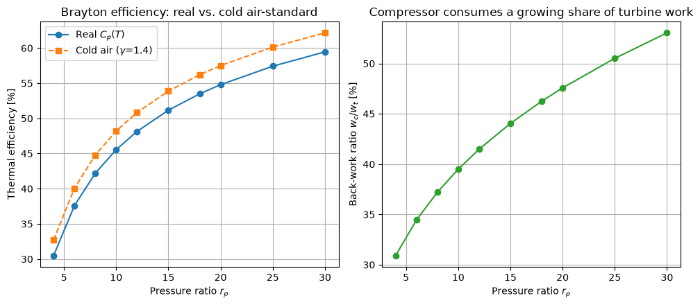
The cold air-standard formula \(\eta = 1 - r_p^{(1-\gamma)/\gamma}\) predicts monotonically increasing efficiency. With real \(C_p(T)\), the efficiency curve is similar in shape but shifted because \(\gamma(T)\) decreases as temperature rises (vibrational modes unlock), making the compressor “stiffer” and the turbine less effective at higher pressure ratios than the cold-air approximation suggests.
[8]:
rp_range = np.array([4, 6, 8, 10, 12, 15, 18, 20, 25, 30])
eta_real_list = []
eta_cold_list = []
backwork_list = []

with ThermochemicalCalculator() as calc:
    for rp in rp_range:
        st = brayton_states(calc, T1=300.0, T3=1400.0, rp=rp)
        _, h1 = st["1 (compressor inlet)"]
        _, h2 = st["2 (compressor outlet)"]
        _, h3 = st["3 (turbine inlet)"]
        _, h4 = st["4 (turbine outlet)"]
        w_comp = h2 - h1
        w_turb = h3 - h4
        q_in   = h3 - h2
        eta_real_list.append((w_turb - w_comp) / q_in * 100)
        eta_cold_list.append((1 - rp ** ((1 - 1.4) / 1.4)) * 100)
        backwork_list.append(w_comp / w_turb * 100)

fig, (ax1, ax2) = plt.subplots(1, 2, figsize=(10, 4.5))

ax1.plot(rp_range, eta_real_list, "o-", label="Real $C_p(T)$")
ax1.plot(rp_range, eta_cold_list, "s--", label=r"Cold air ($\gamma$=1.4)")
ax1.set_xlabel("Pressure ratio $r_p$")
ax1.set_ylabel("Thermal efficiency [%]")
ax1.set_title("Brayton efficiency: real vs. cold air-standard")
ax1.legend()

ax2.plot(rp_range, backwork_list, "o-", color="C2")
ax2.set_xlabel("Pressure ratio $r_p$")
ax2.set_ylabel("Back-work ratio $w_c / w_t$ [%]")
ax2.set_title("Compressor consumes a growing share of turbine work")

plt.tight_layout()
plt.show()
Summary
Real \(C_p(T)\) from
pyglennenables accurate Brayton-cycle analysis without assuming constant \(\gamma\).The isentropic condition \(s^\circ(T_2) = s^\circ(T_1) + R\ln(P_2/P_1)\) is solved numerically for each process.
The real efficiency curve is close to but distinct from the cold-air ideal; the difference grows at higher pressure ratios where \(\gamma(T)\) deviates from 1.4.
The back-work ratio (compressor work / turbine work) rises with \(r_p\), limiting practical pressure ratios for single-shaft engines.
Next: notebook 10 shows how to use pyglenn as a high-performance property provider for CFD and chemical kinetics codes.