07 - Comparing Fuels & Biofuels
The package’s design notes (ideias.md, Dr. Reginaldo G. Leão Jr., GESESC / IFMG) call out a concrete research use case: comparing the thermodynamic performance of ethanol, gasoline and sustainable aviation fuel (SAF). This notebook builds that comparison on top of pyglenn.
We evaluate six energy carriers spanning renewable and fossil sources:
symbol |
species |
role |
|---|---|---|
H₂ |
|
green hydrogen |
CH₄ |
|
natural gas / biomethane |
CH₃OH |
|
methanol |
C₂H₅OH |
|
bioethanol |
iso-C₈H₁₈ |
|
gasoline surrogate |
Jet-A |
|
kerosene / SAF surrogate (≈ C₁₂H₂₃) |
For each we compute the heating value, energy density, stoichiometric air demand and carbon intensity.
[1]:
from pyglenn import ThermochemicalCalculator, R

print("Universal gas constant R =", R, "J/(mol.K)")
Universal gas constant R = 8.314462618 J/(mol.K)
[2]:
%matplotlib inline
import numpy as np
import matplotlib.pyplot as plt
import pandas as pd

plt.rcParams["figure.figsize"] = (8, 4.5)
plt.rcParams["axes.grid"] = True
pd.set_option("display.float_format", lambda v: f"{v:,.3f}")
1. Combustion metrics for a general fuel \(C_xH_yO_z\)
Complete combustion is
From pyglenn we get the LHV (gaseous water); from the molar mass we get the gravimetric energy density; the air demand and CO₂ output follow from stoichiometry. Air is 21 % O₂ by mole, mean molar mass 28.97 g/mol.
[3]:
AIR_M = 28.97          # g/mol
CO2_M = 44.01          # g/mol
O2_PER_AIR = 0.21

FUELS = {
    "H2":              dict(species="H2",              x=0, y=2,  z=0),
    "CH4":             dict(species="CH4",             x=1, y=4,  z=0),
    "CH3OH":           dict(species="CH3OH",           x=1, y=4,  z=1),
    "C2H5OH":          dict(species="C2H5OH",          x=2, y=6,  z=1),
    "isooctane":       dict(species="C8H18,isooctane", x=8, y=18, z=0),
    "Jet-A":           dict(species="Jet-A(g)",        x=12, y=23, z=0),
}

def molar_mass(calc, name):
    sid = calc.get_available_species(name, exact_match=True)[0]["id"]
    return calc.db.get_species_data(sid)["molecular_weight"]

def combustion_metrics(calc, species, x, y, z):
    nO2 = x + y / 4 - z / 2
    def H(name, nu, T=298.15):
        return nu * calc.calculate_properties(calc.get_available_species(name, exact_match=True)[0]["id"], T)["h_relative"]
    dh = (H("CO2", x) + H("H2O", y / 2)) - (H(species, 1) + H("O2", nO2))
    lhv = -dh                                   # J/mol
    M = molar_mass(calc, species)               # g/mol
    n_air = nO2 / O2_PER_AIR                     # mol air per mol fuel
    afr_mass = n_air * AIR_M / M                 # kg air / kg fuel
    lhv_MJ_per_kg = lhv / M / 1000.0
    co2_g_per_MJ = (x * CO2_M) / (lhv / 1e6)     # g CO2 per MJ fuel energy
    return dict(M=M, LHV_kJ_mol=lhv / 1000.0, LHV_MJ_kg=lhv_MJ_per_kg,
                AFR=afr_mass, CO2_g_per_MJ=co2_g_per_MJ)
2. The comparison table
[4]:
rows = {}
with ThermochemicalCalculator() as calc:
    for label, f in FUELS.items():
        rows[label] = combustion_metrics(calc, **f)

fuel_df = pd.DataFrame(rows).T
fuel_df = fuel_df.rename(columns={
    "M": "M [g/mol]", "LHV_kJ_mol": "LHV [kJ/mol]", "LHV_MJ_kg": "LHV [MJ/kg]",
    "AFR": "stoich. AFR [-]", "CO2_g_per_MJ": "CO2 [g/MJ]",
})
print(fuel_df.to_string())
           M [g/mol]  LHV [kJ/mol]  LHV [MJ/kg]  stoich. AFR [-]  CO2 [g/MJ]
H2             2.016       241.825      119.960           34.216       0.000
CH4           16.042       802.557       50.027           17.198      54.837
CH3OH         32.042       676.218       21.104            6.458      65.083
C2H5OH        46.068     1,277.541       27.731            8.984      68.898
isooctane    114.229     5,100.475       44.652           15.096      69.029
Jet-A        167.311     7,253.421       43.353           14.635      72.810
3. Gravimetric energy density
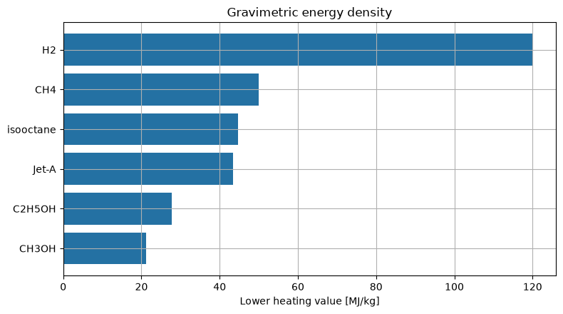
Hydrogen dwarfs every carbon fuel per unit mass; the oxygenated biofuels (methanol, ethanol) carry less energy per kilogram than gasoline or kerosene because the fuel molecule already contains oxygen.
[5]:
order = fuel_df.sort_values("LHV [MJ/kg]", ascending=True)
fig, ax = plt.subplots()
ax.barh(order.index, order["LHV [MJ/kg]"], color="#2471a3")
ax.set_xlabel("Lower heating value [MJ/kg]")
ax.set_title("Gravimetric energy density")
fig.tight_layout()
plt.show()
4. Carbon intensity
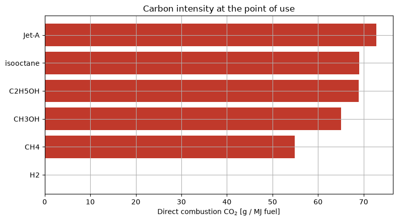
Direct combustion CO₂ per unit of delivered energy. Hydrogen emits none at the point of use; methane is the least carbon-intensive hydrocarbon (high H:C ratio).
Life-cycle caveat. These are direct combustion emissions. Biogenic fuels (bioethanol, biomethane, SAF from biomass) recycle atmospheric CO₂, so their net life-cycle carbon can be far lower than the bar shown here — a central theme of GESESC’s renewable-energy work.
[6]:
order = fuel_df.sort_values("CO2 [g/MJ]", ascending=True)
colors = ["#27ae60" if v == 0 else "#c0392b" for v in order["CO2 [g/MJ]"]]
fig, ax = plt.subplots()
ax.barh(order.index, order["CO2 [g/MJ]"], color=colors)
ax.set_xlabel("Direct combustion CO$_2$ [g / MJ fuel]")
ax.set_title("Carbon intensity at the point of use")
fig.tight_layout()
plt.show()
5. Stoichiometric air-fuel ratio
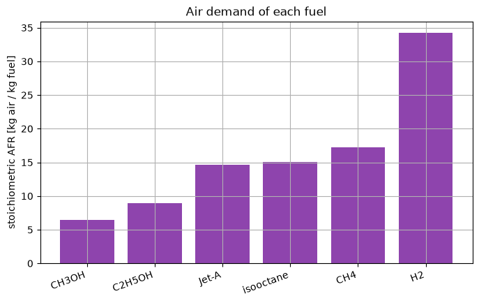
The AFR sizes the air handling of an engine or combustor. Hydrogen and the pure hydrocarbons need a lot of air per kilogram of fuel; oxygenated fuels need less because they carry their own oxygen — relevant to flame speed and NOₓ formation.
[7]:
order = fuel_df.sort_values("stoich. AFR [-]", ascending=True)
fig, ax = plt.subplots()
ax.bar(order.index, order["stoich. AFR [-]"], color="#8e44ad")
ax.set_ylabel("stoichiometric AFR [kg air / kg fuel]")
ax.set_title("Air demand of each fuel")
plt.setp(ax.get_xticklabels(), rotation=20, ha="right")
plt.show()
6. Heating value vs. temperature
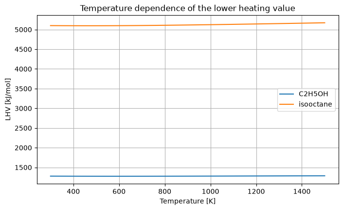
For ethanol and isooctane we trace how the LHV drifts with temperature (Kirchhoff’s law, notebook 05). The change is small — a few percent — confirming that room-temperature heating values are usable across combustor-relevant temperatures.
[8]:
def lhv_at_T(calc, f, T):
    x, y, z = f["x"], f["y"], f["z"]
    nO2 = x + y / 4 - z / 2
    def H(name, nu):
        return nu * calc.calculate_properties(calc.get_available_species(name, exact_match=True)[0]["id"], T)["h_relative"]
    dh = (H("CO2", x) + H("H2O", y / 2)) - (H(f["species"], 1) + H("O2", nO2))
    return -dh / 1000.0

Tgrid = np.linspace(300, 1500, 40)
fig, ax = plt.subplots()
with ThermochemicalCalculator() as calc:
    for label in ["C2H5OH", "isooctane"]:
        f = FUELS[label]
        lhv = [lhv_at_T(calc, f, T) for T in Tgrid]
        ax.plot(Tgrid, lhv, label=label)
ax.set_xlabel("Temperature [K]")
ax.set_ylabel("LHV [kJ/mol]")
ax.set_title("Temperature dependence of the lower heating value")
ax.legend()
plt.show()
Conclusion
Bioethanol / methanol: renewable and clean-burning, but ~35–50 % lower energy density than gasoline — acceptable for ground transport, penalising for aviation.
Isooctane / Jet-A: high gravimetric and volumetric energy density — hence the drive for drop-in SAF that matches kerosene’s properties while cutting life-cycle carbon.
Hydrogen: unmatched energy per kilogram and zero point-of-use CO₂, but its storage and air-demand characteristics differ sharply from liquid fuels.
pyglenn makes such trade-off screening a few lines of code — exactly the rapid, programmatic access to thermochemical data the design notes advocate.
Next: notebook 08 turns to chemical equilibrium and Gibbs energy.