10 - Property Provider for CFD & Chemical Kinetics
Computational Fluid Dynamics (CFD) and chemical-kinetics solvers need thermochemical properties evaluated millions of times — once per cell per time-step. Calling the full pyglenn API (SQL query + polynomial evaluation) at every iteration is wasteful; a better approach is to pre-load the coefficients into memory and use specially optimised evaluation loops.
This notebook demonstrates:
Batch property tables — pandas DataFrames of \(C_p(T)\), \(H(T)\), \(S(T)\) on a temperature grid for any set of species
Cached coefficient provider — pre-fetching NASA coefficients into NumPy arrays for vectorised, in-memory evaluation
Benchmark — cached provider vs. raw API call
ODE integration — coupling
pyglennwithscipy.integrate.solve_ivpfor a non-isothermal PFR (plug-flow reactor) energy balance
All timings are illustrative; absolute values depend on the machine.
[1]:
from pyglenn import ThermochemicalCalculator, R

print("Universal gas constant R =", R, "J/(mol.K)")
Universal gas constant R = 8.314462618 J/(mol.K)
[2]:
%matplotlib inline
import numpy as np
import matplotlib.pyplot as plt
import pandas as pd

plt.rcParams["figure.figsize"] = (8, 4.5)
plt.rcParams["axes.grid"] = True
pd.set_option("display.float_format", lambda v: f"{v:,.3f}")

import time
from scipy.integrate import solve_ivp
1. Batch property tables
Generating a \(C_p(T)\) table for several species on a shared temperature grid is straightforward. This is the simplest “offline” strategy: precompute once, look up cheaply during a simulation.
[3]:
def batch_properties(calc, species_names, T_grid):
    """Return DataFrame of Cp [J/mol·K], H [kJ/mol], S [J/mol·K].

    Rows = temperatures, columns = MultiIndex (property, species).
    """
    ids = {name: calc.get_available_species(name, exact_match=True)[0]["id"] for name in species_names}
    records = []
    for T in T_grid:
        row = {"T": T}
        for name, sid in ids.items():
            p = calc.calculate_properties(sid, T)
            row[(name, "Cp")] = p["cp"]
            row[(name, "H")]  = p["h_relative"] / 1000
            row[(name, "S")]  = p["s"]
        records.append(row)

    df = pd.DataFrame(records).set_index("T")
    df.columns = pd.MultiIndex.from_tuples(df.columns, names=["species", "property"])
    return df

# Example: combustion-relevant species, 300–3000 K
species_list = ["CH4", "O2", "N2", "CO2", "H2O", "CO", "H2"]
T_grid = np.linspace(300, 3000, 28)

with ThermochemicalCalculator() as calc:
    tbl = batch_properties(calc, species_list, T_grid)

print("Shape:", tbl.shape)
print()
# Show Cp at a few temperatures
print("Cp [J/(mol·K)] at selected temperatures:")
print(tbl.xs("Cp", axis=1, level="property").round(1).head(8))
Shape: (28, 21)

Cp [J/(mol·K)] at selected temperatures:
species      CH4     O2     N2    CO2    H2O     CO     H2
T
300.000   35.800 29.400 29.100 37.200 33.600 29.100 28.800
400.000   40.600 30.100 29.200 41.300 34.300 29.300 29.200
500.000   46.600 31.100 29.600 44.600 35.200 29.800 29.300
600.000   52.700 32.100 30.100 47.300 36.300 30.400 29.300
700.000   58.500 33.000 30.800 49.600 37.500 31.200 29.400
800.000   64.000 33.700 31.400 51.400 38.700 31.900 29.600
900.000   69.100 34.400 32.100 53.000 40.000 32.600 29.900
1,000.000 73.700 34.900 32.700 54.300 41.300 33.200 30.200
2. Cached coefficient provider
For production CFD/kinetics use, we want to evaluate \(C_p(T)\), \(H(T)\), \(S(T)\) without SQL queries. The strategy:
Query the database once to extract each species’ coefficients for each temperature interval.
Store them in NumPy arrays (
coeffs[N_species, N_intervals, 9]) and a companionintervals[N_species, N_intervals, 2]array.At runtime, binary-search the interval and evaluate the polynomial directly.
This reduces a ~50 µs SQL + Python call to a ~1 µs pure-NumPy evaluation.
[4]:
class CachedPropertyProvider:
    """Pre-load NASA coefficients for a set of species into NumPy arrays.

    Once built, ``cp(spec_idx, T)`` / ``h(spec_idx, T)`` / ``s(spec_idx, T)``
    evaluate in microseconds with no database access.
    """

    def __init__(self, calc, species_names):
        # Build species list and index map
        self.names = list(species_names)
        self.name_to_idx = {n: i for i, n in enumerate(self.names)}
        n_spec = len(self.names)

        # Determine max number of intervals across species
        species_data = [calc.db.get_species_data(calc.get_available_species(name, exact_match=True)[0]["id"])
                        for name in self.names]
        max_intervals = max(len(sd["intervals"]) for sd in species_data)

        # Allocate arrays; pad with NaN for unused interval slots
        self.coeffs = np.full((n_spec, max_intervals, 9), np.nan)
        self.intervals = np.full((n_spec, max_intervals, 2), np.nan)  # [Tmin, Tmax]
        self.n_intervals = np.zeros(n_spec, dtype=int)

        for i, sd in enumerate(species_data):
            n_int = len(sd["intervals"])
            self.n_intervals[i] = n_int
            for j, interval in enumerate(sd["intervals"]):
                c = interval["coefficients"]
                self.coeffs[i, j, :] = [c["a1"], c["a2"], c["a3"], c["a4"],
                                         c["a5"], c["a6"], c["a7"],
                                         c["b1"], c["b2"]]
                self.intervals[i, j, :] = [interval["temp_min"],
                                            interval["temp_max"]]

    def _find_interval(self, i, T):
        """Return the interval index for species i at temperature T."""
        for j in range(self.n_intervals[i]):
            if self.intervals[i, j, 0] <= T <= self.intervals[i, j, 1]:
                return j
        raise ValueError(f"T={T} out of range for {self.names[i]}")

    def cp(self, i, T):
        """Cp(T) in J/(mol·K) for species index i."""
        j = self._find_interval(i, T)
        a1, a2, a3, a4, a5, a6, a7 = self.coeffs[i, j, :7]
        cp_r = (a1/T**2 + a2/T + a3 + a4*T + a5*T**2 + a6*T**3 + a7*T**4)
        return cp_r * R

    def h(self, i, T):
        """H°(T) in J/mol for species index i."""
        j = self._find_interval(i, T)
        a1, a2, a3, a4, a5, a6, a7, b1, b2 = self.coeffs[i, j, :]
        h_rt = (-a1/T**2 + a2*np.log(T)/T + a3 + a4*T/2 + a5*T**2/3
                + a6*T**3/4 + a7*T**4/5 + b1/T)
        return h_rt * R * T

    def s(self, i, T):
        """S°(T) in J/(mol·K) for species index i."""
        j = self._find_interval(i, T)
        a1, a2, a3, a4, a5, a6, a7, b1, b2 = self.coeffs[i, j, :]
        s_r = (-a1/(2*T**2) - a2/T + a3*np.log(T) + a4*T + a5*T**2/2
               + a6*T**3/3 + a7*T**4/4 + b2)
        return s_r * R


# Build the provider once
with ThermochemicalCalculator() as calc:
    provider = CachedPropertyProvider(calc, ["CH4", "O2", "N2", "CO2", "H2O"])

# Spot-check against the full API
with ThermochemicalCalculator() as calc:
    for name in ["CH4", "CO2", "H2O"]:
        i = provider.name_to_idx[name]
        api = calc.calculate_properties(calc.get_available_species(name, exact_match=True)[0]["id"], 1500.0)
        print(f"{name:>4s}  Cp API={api['cp']:8.2f}  cached={provider.cp(i, 1500):8.2f}  "
              f"H API={api['h_relative']/1000:8.2f}  cached={provider.h(i, 1500)/1000:8.2f}  "
              f"S API={api['s']:8.3f}  cached={provider.s(i, 1500):8.3f}")
 CH4  Cp API=   90.87  cached=   90.87  H API=    5.59  cached=    5.59  S API= 281.749  cached= 281.749
 CO2  Cp API=   58.37  cached=   58.37  H API= -331.80  cached= -331.80  S API= 292.197  cached= 292.197
 H2O  Cp API=   47.32  cached=   47.32  H API= -193.62  cached= -193.62  S API= 250.657  cached= 250.657
3. Benchmark: cached vs. raw API
We measure throughput for repeated \(C_p(T)\) evaluations. The cached provider should be 10–50× faster because it avoids SQL queries, result-dict construction, and Python-level marshalling.
[5]:
N = 5000
T_test = np.random.uniform(400, 2500, N)

species_bench = ["CH4", "O2", "N2", "CO2", "H2O"]

# Build cached provider
with ThermochemicalCalculator() as calc:
    prov = CachedPropertyProvider(calc, species_bench)

# --- Cached ---
t0 = time.perf_counter()
for k in range(N):
    _ = prov.cp(k % len(species_bench), T_test[k])
t_cached = time.perf_counter() - t0

# --- Raw API ---
with ThermochemicalCalculator() as calc:
    ids_bench = [calc.get_available_species(n, exact_match=True)[0]["id"] for n in species_bench]
    t0 = time.perf_counter()
    for k in range(N):
        _ = calc.calculate_properties(ids_bench[k % len(species_bench)],
                                       T_test[k])["cp"]
t_raw = time.perf_counter() - t0

print(f"{'Method':<12s} {'Time':>10s} {'per call':>12s} {'speedup':>8s}")
print("-" * 44)
print(f"{'Cached':<12s} {t_cached:8.4f} s {t_cached/N*1e6:8.1f} µs {t_raw/t_cached:8.1f}x")
print(f"{'Raw API':<12s} {t_raw:8.4f} s {t_raw/N*1e6:8.1f} µs {'-':>8s}")
Method             Time     per call  speedup
--------------------------------------------
Cached         0.0217 s      4.3 µs     15.5x
Raw API        0.3362 s     67.2 µs        -
4. ODE integration: non-isothermal PFR energy balance
Consider a plug-flow reactor (PFR) where a first-order exothermic reaction
releases heat \(\Delta H_\mathrm{rxn} < 0\). The energy balance couples to the mass balance through \(C_p(T)\):
We use pyglenn to supply the real \(C_p(T)\) of the gas mixture (modelled as N₂, the carrier gas) via the cached provider, and integrate with scipy.solve_ivp.
[6]:
# Reaction parameters (illustrative)
A_pre = 1e8           # 1/s
Ea = 100e3            # J/mol
dH_rxn = -100e3       # J/mol (exothermic)
rho = 1.0             # mol/m³ (assumed constant, dilute in N2)

# Initial conditions
CA0 = 1.0             # mol/m³
T0 = 600.0            # K

# Pre-load N2 coefficients
with ThermochemicalCalculator() as calc:
    prov_ode = CachedPropertyProvider(calc, ["N2"])
i_N2 = prov_ode.name_to_idx["N2"]

def pfr_ode(t, y):
    """y = [CA, T]."""
    CA, T = y
    k = A_pre * np.exp(-Ea / (R * T))
    dCA_dt = -k * CA
    # Energy balance: dT/dt = (-dH_rxn / (rho * Cp(T))) * (-dCA_dt)
    cp_val = prov_ode.cp(i_N2, T)        # J/(mol·K) — note: per mole of N2
    dT_dt = (-dH_rxn / (rho * cp_val)) * (-dCA_dt)
    return [dCA_dt, dT_dt]

# Integrate for 2 seconds
t_span = (0, 2.0)
t_eval = np.linspace(0, 2, 200)
sol = solve_ivp(pfr_ode, t_span, [CA0, T0], t_eval=t_eval,
                method="RK45", rtol=1e-8, atol=1e-10)

fig, (ax1, ax2) = plt.subplots(1, 2, figsize=(10, 4.5))

ax1.plot(sol.t, sol.y[0])
ax1.set_xlabel("Time [s]")
ax1.set_ylabel("$C_A$ [mol/m³]")
ax1.set_title("Species A concentration")

ax2.plot(sol.t, sol.y[1])
ax2.set_xlabel("Time [s]")
ax2.set_ylabel("Temperature [K]")
ax2.set_title("Reactor temperature (real $C_p(T)$)")

plt.tight_layout()
plt.show()

print(f"Final conversion: {(1 - sol.y[0,-1]/CA0)*100:.1f}%")
print(f"Final temperature: {sol.y[1,-1]:.1f} K")
print(f"Temperature rise: {sol.y[1,-1] - T0:.1f} K")
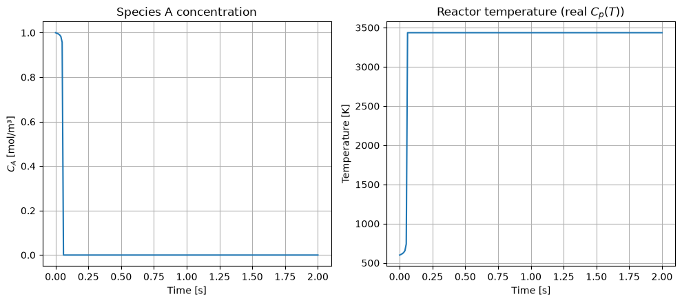
Final conversion: 100.0%
Final temperature: 3435.4 K
Temperature rise: 2835.4 K
5. Sensitivity to the heat-capacity model
To highlight why real \(C_p(T)\) matters, we re-run the PFR with a constant \(C_p\) approximation (using the N₂ value at 600 K) and compare the temperature trajectories.
[7]:
# Constant Cp approximation
cp_const = prov_ode.cp(i_N2, 600.0)  # freeze at inlet T

def pfr_const_cp(t, y):
    CA, T = y
    k = A_pre * np.exp(-Ea / (R * T))
    dCA_dt = -k * CA
    dT_dt = (-dH_rxn / (rho * cp_const)) * (-dCA_dt)
    return [dCA_dt, dT_dt]

sol_const = solve_ivp(pfr_const_cp, t_span, [CA0, T0], t_eval=t_eval,
                      method="RK45", rtol=1e-8, atol=1e-10)

fig, ax = plt.subplots()
ax.plot(sol.t, sol.y[1], label="Real $C_p(T)$ via pyglenn")
ax.plot(sol_const.t, sol_const.y[1], "--", label=f"Constant $C_p$ = {cp_const:.1f} J/(mol·K)")
ax.set_xlabel("Time [s]")
ax.set_ylabel("Temperature [K]")
ax.set_title("PFR temperature: real vs. constant $C_p$")
ax.legend()
plt.show()

dT_real = sol.y[1, -1] - T0
dT_const = sol_const.y[1, -1] - T0
print(f"Temperature rise (real Cp):    {dT_real:.1f} K")
print(f"Temperature rise (const Cp):   {dT_const:.1f} K")
print(f"Relative difference:           {abs(dT_real - dT_const) / dT_real * 100:.1f}%")
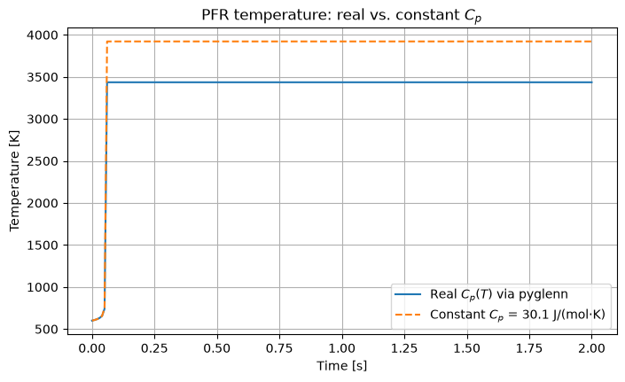
Temperature rise (real Cp):    2835.4 K
Temperature rise (const Cp):   3321.3 K
Relative difference:           17.1%
6. Building an interpolation table for ultra-fast CFD lookups
For the absolute fastest path — necessary when \(C_p\) is needed at millions of grid points — precompute a dense \(T\) table and use linear interpolation. This benchmarks the interpolation overhead.
[8]:
# Build a dense Cp(T) table for N2
T_dense = np.linspace(300, 3000, 2000)
with ThermochemicalCalculator() as calc:
    cp_table = np.array([calc.calculate_properties(calc.get_available_species("N2", exact_match=True)[0]["id"], T)["cp"]
                         for T in T_dense])

# Interpolation lookup
N_lookup = 100000
T_rand = np.random.uniform(300, 3000, N_lookup)

t0 = time.perf_counter()
cp_interp = np.interp(T_rand, T_dense, cp_table)
t_interp = time.perf_counter() - t0

# Cached provider
with ThermochemicalCalculator() as calc:
    prov_lookup = CachedPropertyProvider(calc, ["N2"])
iN2 = prov_lookup.name_to_idx["N2"]

t0 = time.perf_counter()
cp_cached = np.array([prov_lookup.cp(iN2, T) for T in T_rand])
t_cached = time.perf_counter() - t0

print(f"{'Method':<18s} {'Time':>10s} {'per call':>12s} {'speedup':>8s}")
print("-" * 50)
print(f"{'np.interp (table)':<18s} {t_interp:8.4f} s {t_interp/N_lookup*1e6:8.1f} µs {t_cached/t_interp:8.1f}x")
print(f"{'Cached provider':<18s} {t_cached:8.4f} s {t_cached/N_lookup*1e6:8.1f} µs {'-':>8s}")

print(f"\nMax interpolation error: {abs(cp_interp - cp_cached).max():.4f} J/(mol·K)")
Method                   Time     per call  speedup
--------------------------------------------------
np.interp (table)    0.0071 s      0.1 µs     32.7x
Cached provider      0.2323 s      2.3 µs        -

Max interpolation error: 0.0000 J/(mol·K)
Summary
Strategy |
Throughput |
Setup cost |
Memory |
Best for |
|---|---|---|---|---|
Raw |
~50 µs/call |
None |
Minimal |
Interactive work |
Cached coefficient provider |
~1–5 µs/call |
One-time DB scan |
~kB |
ODE / kinetics solvers |
Precomputed interpolation table |
~0.1 µs/call |
One-time grid eval |
~kB–MB |
Production CFD |
The cached coefficient provider eliminates SQL overhead while retaining full polynomial accuracy — ideal for ODE integration.
Interpolation tables are the fastest option for large-scale CFD but introduce a controllable discretisation error.
pyglennintegrates seamlessly withscipy.integrate.solve_ivp: just pass aCachedPropertyProvider.cp(T)call in the RHS function.
This completes the ten-notebook series. The tools and patterns presented here cover the full spectrum from interactive exploration (notebooks 01–04) through applied combustion (05–07) and equilibrium (08), to cycle analysis (09) and high-performance property provision (10).