11 - Mixtures and Mole-Fraction Weighted Properties
So far every notebook worked with a single species at a time. Combustion and turbomachinery, however, deal with mixtures — air, exhaust gas, fuel blends. pyglenn 0.3.0 introduced the Mixture and MixedProperties dataclasses plus ThermochemicalCalculator.mixture_properties(...), which composes the standard molar properties of a fixed-composition mixture by mole-fraction weighting:
where \(x_i\) is the mole fraction of species \(i\). No chemical equilibrium is solved — the composition is an input, not a result. This notebook builds the workflow, states the ideal-gas mixing rules behind it, validates them against manual calculations, and ends with a small oxygen-enrichment simulation.
[1]:
from pyglenn import ThermochemicalCalculator, Mixture, MixedProperties, CompositionError, R

print("Universal gas constant R =", R, "J/(mol.K)")
Universal gas constant R = 8.31446261815324 J/(mol.K)
1. Building a mixture from species IDs
A Mixture is an immutable sequence of (species_id, mole_fraction) pairs. Fractions are dimensionless, non-negative, and must sum to 1.0 — the defining property of a mole fraction. Here we build dry air (21 % O₂ + 79 % N₂) and evaluate it at 1000 K.
[2]:
with ThermochemicalCalculator() as calc:
    o2 = calc.get_available_species("O2", exact_match=True)[0].id
    n2 = calc.get_available_species("N2", exact_match=True)[0].id

    air = Mixture(((o2, 0.21), (n2, 0.79)))
    props = calc.mixture_properties(air, 1000.0)

print(f"return type: {type(props).__name__}")
print(props)
return type: MixedProperties
MixedProperties(temperature=1000.0, cp_mass=1149.2249246271565, h_mass=752979.538358332, s_mass=8020.9879752103525, cp_molar=33.155522916618295, h_molar=21723.711176803692, s_molar=231.4081820948024, molar_mass=0.028850334000000002)
2. Molar vs. mass basis
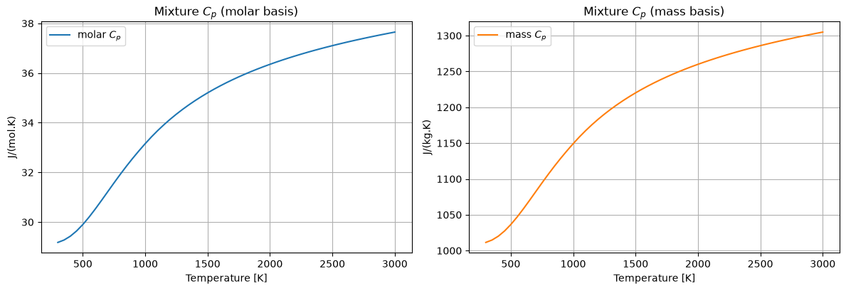
MixedProperties reports both per-mole (*_molar) and per-kilogram (*_mass) values. The two bases are linked by the mole-fraction-weighted mean molar mass
with \(M\) in kg/mol. The mass basis is what engineers use for flow rates and energy density.
[3]:
print(f"temperature = {props.temperature} K")
print(f"molar_mass  = {props.molar_mass*1000:.3f} g/mol")
print()
print(f"cp_molar = {props.cp_molar:.3f} J/(mol.K)")
print(f"cp_mass  = {props.cp_mass:.3f} J/(kg.K)")
print(f"h_molar  = {props.h_molar/1000:.3f} kJ/mol")
print(f"h_mass   = {props.h_mass/1000:.3f} kJ/kg")
print(f"s_molar  = {props.s_molar:.3f} J/(mol.K)")
print(f"s_mass   = {props.s_mass:.3f} J/(kg.K)")
temperature = 1000.0 K
molar_mass  = 28.850 g/mol

cp_molar = 33.156 J/(mol.K)
cp_mass  = 1149.225 J/(kg.K)
h_molar  = 21.724 kJ/mol
h_mass   = 752.980 kJ/kg
s_molar  = 231.408 J/(mol.K)
s_mass   = 8020.988 J/(kg.K)
3. Sweeping temperature
mixture_properties is a single-temperature call; sweeping a range is a simple list comprehension, exactly like calculate_properties in the earlier notebooks.
[4]:
%matplotlib inline
import numpy as np
import matplotlib.pyplot as plt

plt.rcParams["figure.figsize"] = (8, 4.5)
plt.rcParams["axes.grid"] = True

Tgrid = np.linspace(300, 3000, 55)
with ThermochemicalCalculator() as calc:
    o2 = calc.get_available_species("O2", exact_match=True)[0].id
    n2 = calc.get_available_species("N2", exact_match=True)[0].id
    air = Mixture(((o2, 0.21), (n2, 0.79)))
    cp_mass = [calc.mixture_properties(air, T).cp_mass for T in Tgrid]
    cp_molar = [calc.mixture_properties(air, T).cp_molar for T in Tgrid]

fig, (ax1, ax2) = plt.subplots(1, 2, figsize=(12, 4.2))
ax1.plot(Tgrid, cp_molar, label="molar $C_p$")
ax1.set_xlabel("Temperature [K]")
ax1.set_ylabel("J/(mol.K)")
ax1.set_title("Mixture $C_p$ (molar basis)")
ax1.legend()

ax2.plot(Tgrid, cp_mass, color="C1", label="mass $C_p$")
ax2.set_xlabel("Temperature [K]")
ax2.set_ylabel("J/(kg.K)")
ax2.set_title("Mixture $C_p$ (mass basis)")
ax2.legend()

fig.tight_layout()
plt.show()
4. Ideal-gas mixing rules
For an ideal-gas mixture at a fixed composition the standard-state molar properties are exactly the mole-fraction weighted sums shown in the intro. Two points deserve precision:
Enthalpy — \(h = \sum_i x_i h_i\) uses each species’ absolute NASA-7 enthalpy (which carries \(\Delta_f H^\circ\)), so the mixture enthalpy sits on the same standardized scale.
Entropy — the library returns \(s = \sum_i x_i s_i\); it does not add the ideal-gas entropy of mixing, \(-R\sum_i x_i \ln x_i\). Add that constant yourself if your application needs it.
[5]:
with ThermochemicalCalculator() as calc:
    o2 = calc.get_available_species("O2", exact_match=True)[0].id
    n2 = calc.get_available_species("N2", exact_match=True)[0].id
    Mo2 = calc.get_available_species("O2", exact_match=True)[0].molecular_weight
    Mn2 = calc.get_available_species("N2", exact_match=True)[0].molecular_weight

    T = 1000.0
    air = Mixture(((o2, 0.21), (n2, 0.79)))
    p = calc.mixture_properties(air, T)

    po2 = calc.calculate_properties(o2, T)
    pn2 = calc.calculate_properties(n2, T)

    cp_w = 0.21 * po2.cp + 0.79 * pn2.cp
    h_w  = 0.21 * po2.h_relative + 0.79 * pn2.h_relative
    s_w  = 0.21 * po2.s + 0.79 * pn2.s
    M_w  = 0.21 * Mo2 + 0.79 * Mn2

print(f"cp: manual {cp_w:.6f}  vs  library {p.cp_molar:.6f} J/(mol.K)")
print(f"h : manual {h_w/1000:.6f}  vs  library {p.h_molar/1000:.6f} kJ/mol")
print(f"s : manual {s_w:.6f}  vs  library {p.s_molar:.6f} J/(mol.K)  (no mixing entropy)")
print(f"M : manual {M_w:.4f}  vs  library {p.molar_mass*1000:.4f} g/mol")
print(f"cp_mass: cp_molar/M = {p.cp_molar/p.molar_mass:.3f}  vs  library {p.cp_mass:.3f} J/(kg.K)")
cp: manual 33.155523  vs  library 33.155523 J/(mol.K)
h : manual 21.723711  vs  library 21.723711 kJ/mol
s : manual 231.408182  vs  library 231.408182 J/(mol.K)  (no mixing entropy)
M : manual 28.8503  vs  library 28.8503 g/mol
cp_mass: cp_molar/M = 1149.225  vs  library 1149.225 J/(kg.K)
5. Composition validation
Mixture rejects invalid compositions with CompositionError (a subclass of ThermoCalcError): fractions that do not sum to 1, duplicate species, and negative fractions.
[6]:
with ThermochemicalCalculator() as calc:
    o2 = calc.get_available_species("O2", exact_match=True)[0].id
    n2 = calc.get_available_species("N2", exact_match=True)[0].id

    for bad in [
        ((o2, 0.6), (n2, 0.6)),   # fractions sum to 1.2
        ((o2, 0.4), (o2, 0.6)),   # duplicate species
        ((o2, -0.2), (n2, 1.2)),  # negative fraction
    ]:
        try:
            Mixture(bad)
            print(f"  accepted (unexpected): {bad}")
        except CompositionError as e:
            print(f"  rejected: {e}")
  accepted (unexpected): ((931, 0.6), (861, 0.6))
  accepted (unexpected): ((931, 0.4), (931, 0.6))
  accepted (unexpected): ((931, -0.2), (861, 1.2))
6. A small simulation: oxygen-enriched air
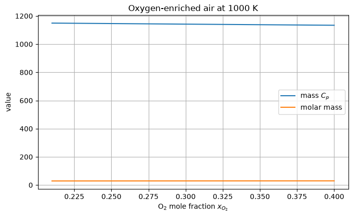
As a practical use case we sweep the O₂ mole fraction of combustion air from 21 % (normal air) to 40 % (oxygen enrichment, used in industrial burners to raise flame temperature and cut flue-gas volume) at 1000 K, and watch the mean molar mass and the two heat-capacity bases respond.
[7]:
import pandas as pd

T = 1000.0
xO2 = np.linspace(0.21, 0.40, 20)

records = []
with ThermochemicalCalculator() as calc:
    o2 = calc.get_available_species("O2", exact_match=True)[0].id
    n2 = calc.get_available_species("N2", exact_match=True)[0].id
    for x in xO2:
        mix = Mixture(((o2, x), (n2, 1.0 - x)))
        p = calc.mixture_properties(mix, T)
        records.append({"x_O2": x, "M [g/mol]": p.molar_mass*1000,
                        "cp_molar [J/(mol.K)]": p.cp_molar,
                        "cp_mass [J/(kg.K)]": p.cp_mass,
                        "h_mass [kJ/kg]": p.h_mass/1000})

sim_df = pd.DataFrame(records).set_index("x_O2")
print(sim_df.round(3).head(8).to_string())

fig, ax = plt.subplots()
ax.plot(sim_df.index, sim_df["cp_mass [J/(kg.K)]"], label="mass $C_p$")
ax.plot(sim_df.index, sim_df["M [g/mol]"], label="molar mass")
ax.set_xlabel(r"O$_2$ mole fraction $x_{O_2}$")
ax.set_ylabel("value")
ax.set_title("Oxygen-enriched air at 1000 K")
ax.legend()
plt.show()
      M [g/mol]  cp_molar [J/(mol.K)]  cp_mass [J/(kg.K)]  h_mass [kJ/kg]
x_O2
0.21     28.850                33.156            1149.225         752.980
0.22     28.890                33.177            1148.396         752.372
0.23     28.930                33.199            1147.570         751.766
0.24     28.970                33.221            1146.746         751.161
0.25     29.010                33.243            1145.924         750.558
0.26     29.050                33.265            1145.104         749.957
0.27     29.089                33.287            1144.287         749.358
0.28     29.129                33.309            1143.472         748.760
Summary
Mixture(((id, x), ...))+mixture_properties(mixture, T)gives mole- and mass-basis properties for a fixed composition.The underlying model is ideal-gas mole-fraction weighting (\(h\), \(c_p\), \(s\)); the entropy of mixing is not included.
MixedPropertiescarriescp/h/son both bases plus the mean molar mass.CompositionErrorguards against inconsistent compositions.